Anomaly Detection in Machine Learning: Classification Algorithms vs Anomaly Detection

Data is the new gold and organizations are harnessing its potential to make the best of this invaluable resource. As organizations gather increasingly large data sets with potential insights into their business activities, identifying anomalous data or outliers becomes crucial. Detecting these anomalies helps uncover inefficiencies, rare events, root causes of issues, and opportunities for operational improvements.

But what are anomalies?

Anomaly means something unusual or abnormal. We often encounter anomalies in our daily life. It can be suspicious activities of an end-user on a network or malfunctioning of equipment. Sometimes it is vital to detect such anomalies to prevent a disaster. For example, detecting a bad user can prevent online fraud, or detecting malfunctioning equipment can prevent system failure.

What is anomaly detection?

Real-world data sets are bound to contain anomalies also known as outlier data points. The reason for this could be any. Sometimes there are anomalies due to corrupted data or human error. However, it is important to note that anomalies can hamper business performance, making it crucial to free your data sets from any anomalies.

On the technical front, anomaly detection is a task related to data that deploys algorithms to identify any abnormal or unusual patterns in data. It is important to do so to keep misrepresentation of data and any other data-related issues at bay. On the bright side, successful anomaly detection can help businesses in various ways, right from reducing costs to managing time to retaining customers. Today more and more businesses are deploying machine learning techniques for anomaly detection to fasten the rate at which anomalies are detected and used for a business advantage. Our blog is curated to help you get a fair idea about different categories of anomalies, the difference between classification algorithms and anomaly detection, and more.

Different Categories of Anomalies:

Anomalies can be divided into three broad categories:

Point Anomaly: This occurs when a single data point notably differs from the rest of the dataset.

Contextual Anomaly: This is identified when an observation appears anomalous due to the specific context in which it occurs.

Collective Anomaly: This type of anomaly is detected when a group of data instances together indicates an abnormal pattern.

Two Powerful Anomaly Detection Techniques

Banking on the right anomaly detection technique largely depends on the type of data that is being used along with how much data has labels versus data that is unlabeled. Primarily anomaly detection techniques fall under supervised and unsupervised categories. Let’s find out what these mean and their significance in anomaly detection.

1. Unsupervised Anomaly Detection

Unsupervised anomaly detection in machine learning is one of the most popular approaches. The reason behind this is that unlabeled anomalous data is more common and works in favor of the unsupervised anomaly detection algorithm to independently make discoveries as there is no need for labels.  In deep learning, techniques like artificial neural networks, isolation forests, and one-class support vector machines are commonly used for anomaly detection. This unsupervised approach is often applied in fields such as fraud detection and medical anomaly identification.

2. Supervised Anomaly Detection

Unlike unsupervised anomaly detection, supervised anomaly detection requires labeled data. The drawback of this technique is that this algorithm can detect anomalies that it has come across before in its training data. This means, the algorithm needs to be fed with enough examples of anomalies and data. Some of the famous industry applications for this technique are detection of fraudulent transactions and detection of manufacturing defects.

Understanding the basics of anomaly detection and its different categories, now let us explore about classification algorithm and anomaly detection.

Classification Algorithms vs Anomaly Detection:

Machine learning provides us with many techniques to classify things, for example, we have algorithms like logistic regression and support vector machines for classification problems. However, these algorithms fail to classify anomalous and non-anomalous problems. In a typical classification problem, we have almost an equal or a comparable number of positive and negative examples. If we have a classification problem, we must decide if a vehicle is a car or not. Then in our dataset the share of cars may be 40-60%, similarly, the share of non-car examples may be 40-60%. So, we generally have a balanced amount of positive and negative examples, and we train our model on a good amount of positive as well as negative examples. On the other hand, in anomaly detection problems we have a significantly lesser amount of positive (anomalous) examples than the negative (non-anomalous) examples. The positive examples may be less than 5% or even 1% (obviously that is why they are anomalous). In such cases, a classification algorithm cannot be trained well on positive examples. Here comes the anomaly detection algorithm to rescue us.

Anomaly Detection Algorithm:

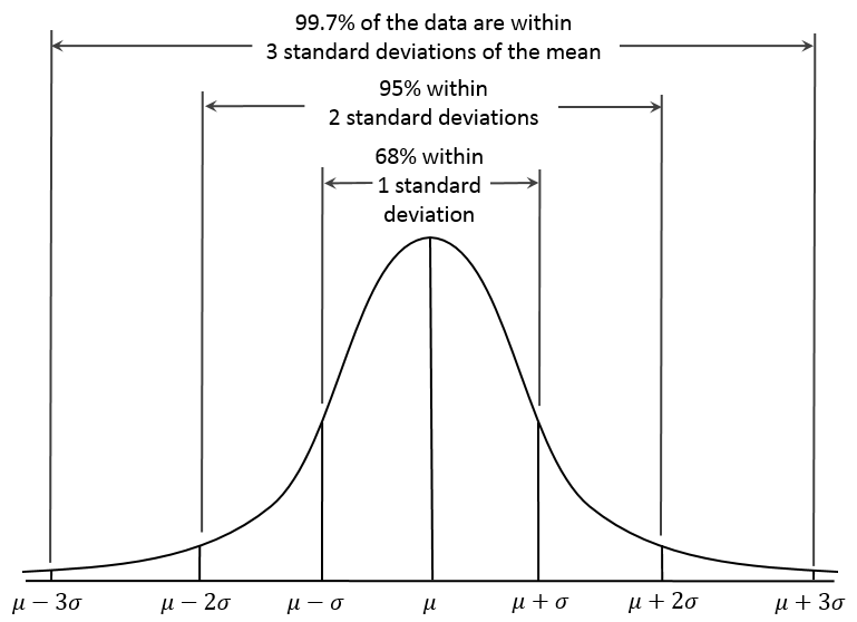
Anomaly detection algorithm works on probability distribution technique. Here we use Gaussian distribution to model our data. It is a bell-shaped function given by

Ɲ (µ, σ²⁾

µ = mean

σ²= Variance

σ = Standard Deviation

If the probability of χ is Gaussian with mean µ and variance  σ²  then

  χ ~ Ɲ (µ, σ² )

‘~’ is called tilde which is read as: “χ is distributed as“.

µ or mean describes the center of the curve.

σ or standard deviation and describes the width of the curve.

The full function is as follows

p(x,  µ, σ²) = (1/ (σ*sqrt(2π)))* e^{– (1/2)*(sqr(x-µ)/σ2)}

Suppose we have data set X as follows

X = [ [ x₁₁   x₁₂  x₁₃  ….. x_1n ]

[ x₂₁   x₂₂  x₂₃  ….. x_2n ]

:

:

:

[ x_m1  x_m2 x_m3 ….. x_mn ] ]

here x_ij  means  j^th feature  i^th  example.

To find mean µ :

We do column-wise summation and divide it by several examples. We get a row matrix of dimension (1x n).

µ = (1/m) * ( Σ^m_i=1  X_i )  ; ( Here subscript i represents column no.)

=  [ [  µ₁   µ₂   µ₃ ……….  µ_n ] ]

To find variance  σ² :

σ² = (1/m) * ( Σ^m_i=1  (x_i – µ)² ) ; (  Here subscript i represents column no. )

In Octave/MATLAB syntax the above expression can be written as

σ² = sum ((X-  µ).^2) * (1/m)

= [  σ²₁   σ²₂   σ²₃ ….   σ²_n  ]

Here we get  σ²  as a row matrix of dimension (1x n).

Algorithm:

Training algorithm

1. Choose features x_i that you think to be indicative of anomalies.
2. Split non-anomalous examples as 60% for training set, 20% for cross-validation, and 20% for the test set.
3. Split anomalous examples as 50% for cross validation set and 50% test set.
4. Calculate µ and σ² on the training set.
   4. Take an arbitrary value as threshold ɛ.
5. Check every example x from the validation set if it is anomalous or not calculate P(x) as follows

P(x)= Πⁿ_j=1 p(x_j ;  µ_{j ;}  σ_j² )

= Πⁿ_j=1{(1/ (σ*sqrt(2π)))* exp(- (1/2)*((x_j-µ_j)² /σ_j²))}

= p(x₁ ;  µ_{1 ;}  σ₁² ) * p(x₂ ;  µ_{2 ;}  σ₂² ) *p(x₃ ;  µ_{3 ;}  σ₃² )*…

……*p(x_n ;  µ_{n ;}  σ_n² )

6. If P(x) is less than threshold ɛ then it is an anomaly otherwise not.
7. Calculate F₁ score for current ɛ.
8. Repeat steps 4,5 and 6 for different values of ɛ and select ɛ which has the highest F₁score

After training, we have µ, σ² and  ɛ .

Algorithm to check whether a new example is an anomaly or not

1. Calculate P(x) for the new examples x as follows:

P(x)= Πⁿ_j=1 p(x_j ;  µ_{j ;}  σ_j² )

= Πⁿ_j=1{(1/ (σ*sqrt(2π)))* exp(- (1/2)*((x_j-µ_j)² /σ_j²))}

= p(x₁ ;  µ_{1 ;}  σ₁² ) * p(x₂ ;  µ_{2 ;}  σ₂² ) *p(x₃ ;  µ_{3 ;}  σ₃² )*…

……*p(x_n ;  µ_{n ;}  σ_n² )

2. If P(x) is less than threshold ɛ then it is an anomaly otherwise not.

F₁ Score:

F₁ score is an error metrics for skewed data. Skewed data is the data where either of positive and negative example is significantly large than the other (>90%).

F₁ score can be given as follows:

F₁ = 2*{(precision * recall)/(precision + recall) }

Where,

precision = True Positive/(True positive + False positive )

recall       = True Positive/(True positive + False negative)

True Positive => When the actual output is +ve and your algorithm predicts +ve

False Positive => When the actual output is -ve and your algorithm predicts +ve

True Negative => When the actual output is -ve and your algorithm predicts -ve

False Negative => When the actual output is +ve and your algorithm predicts -ve

A good algorithm has high precision and recall. F₁ tells us how well our algorithm works. Higher the F1 score the better

Glossary

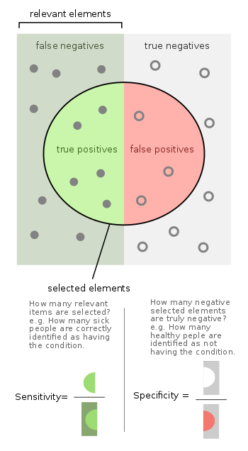
According to medicine and statistics, the terms sensitivity and specificity mathematically represent the accuracy of a particular test regarding presence or absence of a given medical condition. Individuals with the condition are determined as positive and the ones who do not show those conditions are known to be negative. Sensitivity is the metrics to gauge the test’s potential to identify true positives, whereas specificity is the metrics to judge its intensity to identify true negatives.

Sensitivity:

Sensitivity, or the true positive rate, measures the likelihood that a test will correctly identify a positive case when the individual has the condition.

Specificity:

Specificity, or the true negative rate, indicates the probability that a test will accurately produce a negative result when the individual does not have the condition.

When to use Anomaly Detection:

• When we have a very small number of true examples.
• When we have different types of anomalies it is difficult to learn from +ve examples what anomalies look like.

When to use Supervised Learning:

• When we have many both +ve and -ve examples
• When we have enough +ve examples to sense what new +ve example will look like

Choosing what features to use:

The selection of features affects how well your anomaly detection algorithm works. Select those features that are indicative of anomalies. The features you select must be Gaussian. To check whether your features are Gaussian or not, plot them. The plotted graph should be bell-shaped.

If your features are not Gaussian then transform them into Gaussian using any of the functions

• log(x)
• log(x+1)
• log(x+c)
• sqrt(x)
• x^1/3

Final Take

Anomaly detection is inevitable to reap the full potential of data. While traditional and old-school algorithms have their place, they often are unable to identify rare or unusual patterns, this is where anomaly detection algorithms shine.  By using techniques such as Gaussian distribution, it is possible for companies to effectively identify and address anomalies. Furthermore, this can lead to noticeable improvements in operational efficiency, cost reduction, and risk management. It is also essential to understand that the strategic use of machine learning for anomaly detection has the potential to transform data into actionable insights, making sure that businesses stay ahead in a data-driven world. This is why it is essential to choose the right approach and features to harness the power of anomaly detection for your specific needs.

Do you want to get started with anomaly detection by leveraging the potential of Machine Learning?